URL-builder help

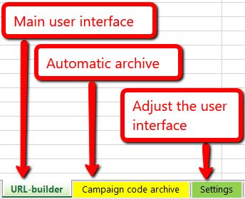
When you have closed the warning(s), you should look at the bottom of the workbook, where the different sheets are listed as tabs.


The two green tabs, are the ones that you should be focusing on now. First you want to make sure, that the tool is setup just to your liking.

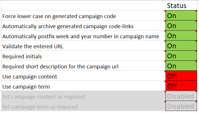
1. Open the "Settings" tab.
2. While letting your mouse hover over each option, make sure that you read what it does.
3. Please select the settings, that would best suit your needs.
   

   By default "campaign content" and "campaign term" are set to off, since they are often not used.

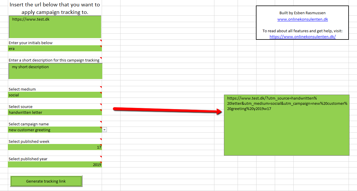
4. Now open the "URL-builder" tab.
5. This is where you generate the UTM tagged campaign URLs.
6. Any displayed but yellow option represents that it is not yet valid.
7. When an option has been filled out correctly and is valid it changes color to green.
8. When all required options have been filled out correctly, the button "Generate tracking link" will turn green.
9. When you click the button and everything is valid the generated campaign URL can be copied from the green text field to the right.
   

   click for full size

1. When you download and open the Workbook, you will probably get a warning like this
2. This is the default warning Excel shows, when trying to open a workbook with custom code.There is nothing harmful in the code whatsoever. It is built to run offline since no external dependencies exist, so while adhering to the guidelines of you organisation, clicking "Enable Content" is required if you want to use all the automation in this tool.

Yes. Each tab/sheet represents a key function in this advanced workbook. If you remove a tab the Campaign URL Builder will stop working.

Yes. Feel free to rename the tabs to something, which is more tailored to your workflow.

Yes. Feel free to rearrange the tabs so they better represent your workflow.

The reason for the option being at the bottom is to force the user to look at all the great existing options before manually adding yet another parameter option.

This is done to minimize the risk of parameter bloat, where similar parameters are added - diluting the efficiency of each similar parameter.

But what you do, is this
If you for example want to switch “Let me add my own” from the bottom of the list to the top, for the UTM parameter “campaign name” you do the following:

1. Open the sheet “Used campaign names”.
2. Find the cell where it says “-1” in the column with the title “Number of times used”.
3. Change “-1” to a number so big that no one parameter will ever be used as much (like a million or so).
4. Save and close the Excel workbook.

Next time you open the workbook, the placement of the “Let me add my own” will have shifted from bottom of the list to the top.

To reverse this, just change it back to -1, then save and close.

This procedure is identical for all UTM parameters, where you want to switch the placement of the “Let me add my own” option from bottom to top.

If you have too many options in a UTM parameter list, I would suggest that you open up the corresponding sheet for this list (if the list represents “source” then open the sheet named “Used source names”).

1. Now highlight row one of the four columns (A1:D1).
2. Apply a filter for the four columns. (“Data” tab –> “Sort and filter” area –> “Filter” button)
   
   

   Click for full size

   
   
3. Make sure that you find an agreeable deletion criteria with your team (Example: parameters before date X with a usage of less than Y).
4. Now apply this criteria via the filter (make sure to remove the tick from “Empty” so you do not accidentally delete the default options – if you want to keep them).
5. When done applying the filters click on the row numbers in the left hand side to highlight the entire rows of the results.
6. When you are done highlighted the results for deletion, right click any one of the highlighted numbers in the left hand side and select “Delete”. This will delete the entire row.
   Deleting the entire rows will not generate any resulting spaces in the list and will therefore ensure that the parameters list keeps working as expected.

You are done

For the nerds:
The reason for deleting the entire row is necessary, is that the tool auto adjusts the scope of the parameters list based on doing a "Ctrl + Shift + down-arrow" to figure out what the last parameter option is. However, this calculation stops when a cell is blank. So in order to avoid blank cells, it is easier to just delete the entire row, when you want to delete a parameter option.